I came across PandasAI while searching for AI integration with Pandas dataframes. My primary objective is to conduct fast exploratory data analysis on new datasets, which would guide my future analysis approach. PandasAI appeared to meet my needs in this regard. In summary, PandasAI is a Python library that seamlessly integrates generative artificial intelligence capabilities (eg Openai) into Pandas, enabling users to perform basic Pandas operations using simple text prompts. It’s worth noting that PandasAI is designed to complement rather than replace Pandas.
What I like about pandasAI
Alternatives LLM integration: Besides openai, PandasAI support integration with Hugging Face’s Starcoder, which is free to use and works pretty well with PandasAI
Return Dataframe Object: PandasAI returns dataframe objects that can be further processed by Pandas or PandasAI itself.
Simplified Plotting process: PandasAI simplifies common plotting tasks for easy data visualization.
In the following sections, we explore a range of common tasks that can be performed by prompting the dataframe instead of the usual pandas operations. We will use a sample dataset “Penguins” loaded from seaborn as our study. We will also be using the Hugging Face starcoder LLM which is free. However, I find that openai is able to deliver the right output with longer and more complex prompt.
!pip install pandasai
# Setting up for prompt import pandas as pd from pandasai import PandasAI from pandasai.llm.starcoder import Starcoder from pandasai.llm.openai import OpenAI import seaborn as sns
# Instantiate a LLM # Openai # llm = OpenAI(api_token="openai_key")
# Starcoder llm = Starcoder(api_token="hugging face api key") pandas_ai = PandasAI(llm)
Basic Operations promptNA operationsFillna and row operations
There are some cases where I did not managed to get an output (openai llm might do a better job) such as below.
# it set to the penguins dataframe instead.
penguins_update = pandas_ai(penguins, prompt= 'return a copy. penguin[ bill_length_mm] = 0 if island = Torgersen', show_code=True)
# Does not return any output
penguins_newcol = pandas_ai(penguins, prompt= 'Add new column "bill_length_cm" by taking "bill_length_mm" /100.')
In conclusion, PandasAI excels at enabling simple and clean exploratory analysis, particularly with its seamless integration of Starcoder, which eliminates cost concerns. However, it may not perform as effectively with longer and more complex prompts, especially when used with Starcoder. It’s important to note that while PandasAI offers valuable functionalities, you will still rely on Pandas for more extensive data manipulation and analysis tasks.
The recommendation is to follow the steps from the original well-written post and refers to the following to fill in some of the possible gaps .
Activate a virtualenv
Git clone the project (in the post) to local directory
Run pip install -r requirements.txt
Upgrade Django version (will encounter error if this step is not performed). pip install django==1.11.17. This only applies if you following the post and cloning the project used in the post.
Create new user in Postgres, create new database & grant assess (Step 1 & 2 of post)
Update settings.py on the database portion.
Create environment variables in the virtualenv. See link for more information.
Note: Secret Key needs to be included as one of the environment variable.
Update the postactivate file of the virtualenv so the environment variables are present when virtualenv is activated.
To get path of the virtualenv: echo $VIRTUAL_ENV
Create new user in Postgres
# Psql codes for Step 1 and 2 of original post.
# ensure Postgres server is running
psql
# create user with password
CREATE USER sample_user WITH PASSWORD 'sample_password';
# create database
CREATE DATABASE sample_database WITH OWNER sample_user;
Update database information in Setting.py
# Changes in the settings.py

DATABASES = {
    'default': {
        'ENGINE': 'django.db.backends.postgresql_psycopg2',
        'NAME': os.environ.get('DB_NAME', ''),
        'USER': os.environ.get('DB_USER', ''),
        'PASSWORD': os.environ.get('DB_PASS', ''),
        'HOST': 'localhost',
        'PORT': '5432',
    }
# SECURITY WARNING: keep the secret key used in production secret!
SECRET_KEY = os.environ.get('DJANGO_SECRET_KEY', '')
Update environment variables in VirtualEnv
# postactivate script in the project virtual env bin path.
# E.g. ~/.virtualenv/[projectname]/bin/postactivate

#!/bin/bash
# This hook is sourced after this virtualenv is activated.
export DB_NAME='sample_database'
export DB_USER='sample_user'
export DB_PASS='sample_password'
export DJANGO_SECRET_KEY='thisissecretkey'
Running migrations (Ensure PostgreSQL server is running)
When running python manage.py runserver on local host and error occurs, check domain is included in the ALLOWED_HOSTS of setting.py. Alternatively, you can use below:
ALLOWED_HOSTS = [‘*’] # for local host only
No database created when running psql command: CREATE DATABASE …, check if semi-colon add to end of the statement. In the event, the ‘;’ is missing, type ‘;’ and try inputting the commands again. See link for more details.
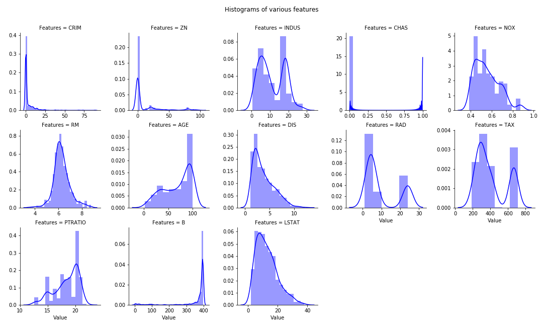
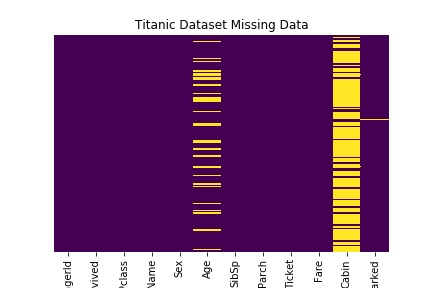
Boston Housing prices dataset is used for 1, 2. Titanic Dataset for item 3.
Basic Python module import
import pandas as pd
import numpy as np
import seaborn as sns
import matplotlib.pyplot as plt
% matplotlib inline

from sklearn.datasets import load_boston
boston = load_boston()
X = boston.data
y = boston.target
df = pd.DataFrame(X, columns= boston.feature_names)
Multiple Histogram plots of numeric features
Stack the dataframe with all the features together. May consume significant memory if dataset have large number of features and observations.
If need to separate by group (hue in FacetGrid), can modify the numeric_features:
Build your own study flash cards video (+ background music) using Python easily.
Required Modules
moviepy
ImageMagick — for creating text clip
pandas — optional for managing CSV file
Basic steps
Read in the text information. Pandas can be used to read in a .csv file for table manipulation.
create a Textclip object for each text and append all Textclips together
Add in an audio if desired. Allow the audio to loop through duration of the clip
Save the file as mp4.
Sample Python Project — Vocabulary flash cards
Below is a simple project to create a vocabulary list of common words use in GMAT etc. For each word and meaning pair, it will flash the word followed by its meaning . There is slight pause in the timing to allow some time for the user to recall on the meaning for the particular words
Sample table for wordlist.csv (which essentially is a table of words and their respective meanings) * random sample (subset) obtained from web
def create_txtclip(tgt_txt, duration = 2, fontsize = 18):
    try:
        txt_clip = TextClip(tgt_txt, fontsize = fontsize, color = 'black',bg_color='white', size=(426,240)).set_duration(duration)
        clip_list.append(txt_clip)
    except UnicodeEncodeError:
        txt_clip = TextClip("Issue with text", fontsize = fontsize, color = 'white').set_duration(2)
        clip_list.append(txt_clip)

from moviepy.editor import *

df = pd.read_csv("wordlist.csv")
for word, meaning in zip(df.iloc[:,0], df.iloc[:,1]):
    create_txtclip(word,1, 70)
    create_txtclip(meaning,3)

final_clip = concatenate(clip_list, method = "compose")

# optional music background with loop
music = AudioFileClip("your_audiofile.mp3")
audio = afx.audio_loop( music, duration=final_clip.duration)

final_clip = final_clip.set_audio(audio)

final_clip.write_videofile("flash_cards.mp4", fps = 24, codec = 'mpeg4')<span id="mce_SELREST_start" style="overflow:hidden;line-height:0;"></span>
In some cases, the audio for the flash cards does not work when play with Quicktime, will work on VLC
This post covers basic PDF manipulation for daily tasks using simple Python modules.
Merging mulitple PDF
Extract text from PDF
Extract image from PDF
Merging PDF
from PyPDF2 import PdfFileMerger
pdfs = ['a.pdf', b.pdf]
merger = PdfFileMerger()

for pdf in pdfs:
    merger.append(pdf)

merger.write("output.pdf")
Extract text from PDF
import pdftotext

# Load your PDF
with open("Target.pdf", "rb") as f:
    pdf = pdftotext.PDF(f)

# Save all text to a txt file.
with open('output.txt', 'w') as f:
    f.write("\n\n".join(pdf))
OR IRkernel::installspec(user = FALSE) #install system-wide
Open a notebook and open new R script.
Further notes
After getting Additional R library might be hard to install inside the Notebook. For workaround, install desired library in R terminal then open the Notebook.
If need to use R.exe on windows command terminal, ensure R.exe is on path. [likely location: C:\R\R-2.15.1\bin]
I created a more generic text cleaning function that can accommodate various text data sets. This can use as a base function for text related problem set. The function, if enabled all options, will be able to perform the following:
Converting all text to lowercase.
Stripping html tags especially if data is scrapped from web.
Replacing accented characters with closest English alphabets/characters.
Removing special characters which includes punctuation. Digits may or may not be excluded depending on context. (Digits are not removed for this data set)
Removing stop-words (simple vs detailed. If detailed, will tokenize words before removal else will use simple word replacement.
Removing extra white spaces and newlines.
Normalize text. This either refer to stemming or lemmatizing.
In this example, we only turn on:
converting text to lowercase
remove special characters (need to keep digits) and white spaces,
do a simple stop words removal.
As mentioned in previous post, it is likely a seller would not include much stop words and will try to keep the title as concise as possible given the limited characters and also to make the title more relevant to search engine. As the text length is not too long, will skip normalizing text to save time.
# Text pre-processing modules
from bs4 import BeautifulSoup
import unidecode
import spacy, en_core_web_sm
nlp = spacy.load('en_core_web_sm', disable=['parser', 'ner'])
from nltk.corpus import stopwords
from nltk.tokenize import word_tokenize
from nltk.stem import PorterStemmer
STOPWORDS = set(stopwords.words('english'))

# Compile regular expression
SPEC_CHARS_REPLACE_BY_SPACE = re.compile('[/(){}\[\]\|@,;]')
SPEC_CHARS = re.compile(r'[^a-zA-z0-9\s]')
SPEC_CHARS_INCLUDE_DIGITS = re.compile(r'[^a-zA-z\s]')
EXTRA_NEWLINES = re.compile(r'[\r|\n|\r\n]+')

## Functions for text preprocessing, cleaning

def strip_htmltags(text):
    soup = BeautifulSoup(text,"lxml")
    return soup.get_text()

def replace_accented_chars(text):
    return unidecode.unidecode(text)

def stem_text(text):
    ps = PorterStemmer()
    modified_txt = ' '.join([ps.stem(word) for word in text.split()])
    return modified_txt

def lemmatize(text):
    modified_text = nlp(text)
    return ' '.join([word.lemma_ if word.lemma_ != '-PRON-' else word.text for word in modified_text])

def normalize(text, method='stem'):
    """ Text normalization to generate the root form of the inflected words.
        This is done by either "stem" or "lemmatize" the text as defined by the 'method' arguments.
        Note that using "lemmatize" will take much longer to run compared to "stem".
    """
    if method == 'stem':
        return stem_text(text)
    if method == 'lemmatize':
        return lemmatize(text)
    print('Please choose either "stem" or "lemmatize" method to normalize.')
    return text

def rm_special_chars(text, rm_digits=False):
    # remove & replace below special chars with space
    modified_txt = SPEC_CHARS_REPLACE_BY_SPACE.sub(' ', text)

    # remove rest of special chars, no replacing with space
    if rm_digits:
        return SPEC_CHARS_INCLUDE_DIGITS.sub('', modified_txt)
    else:
        return SPEC_CHARS.sub('', modified_txt)

def rm_extra_newlines_and_whitespace(text):
    # rm extra newlines
    modified_txt =  EXTRA_NEWLINES.sub(' ', text)

    # rm extra whitespaces
    return re.sub(r'\s+', ' ', modified_txt)

def rm_stopwords(text, simple=True):
    """ Remove stopwords using either the simple model with replacement.
        or using nltk.tokenize to split the words and replace each words. This will incur speed penalty.
    """
    if simple:
        return ' '.join(word for word in text.split() if word not in STOPWORDS)
    else:
        tokens = word_tokenize(text)
        tokens = [token.strip() for token in tokens]
        return ' '.join(word for word in tokens if word not in STOPWORDS)

def clean_text(raw_text, strip_html = True, replace_accented = True,
                normalize_text = True, normalize_methd = 'stem',
                remove_special_chars = True, remove_digits = True,
                remove_stopwords = True, rm_stopwords_simple_mode = True):

    """ The combined function for all the various preprocessing method.
        Keyword args:
            strip_html               : Remove html tags.
            replace_accented         : Convert accented characters to closest English characters.
            normalize_text           : Normalize text based on normalize_methd.
            normalize_methd          : "stem" or "lemmatize". Default "stem".
            remove_special_chars     : Remove special chars.
            remove_digits            : Remove digits/numeric as special characters.
            remove_stopwords         : Stopwords removal basedon NLTK corpus.
            rm_stopwords_simple_mode : skip tokenize before stopword removal. Speed up time.
    """

    text = raw_text.lower()

    if strip_html:
        text = strip_htmltags(text)
    if replace_accented:
        text = replace_accented_chars(text)
    if remove_special_chars:
        text = rm_special_chars(text, remove_digits)
    if normalize_text:
        text = normalize(text, normalize_methd)
    if remove_stopwords:
        text = rm_stopwords(text, rm_stopwords_simple_mode)

    text = rm_extra_newlines_and_whitespace(text)

    return text
Grid Search for Hyper Parameters Tuning
Using pipelines, it is easy to incorporate the sklearn grid search to sweep through the various the hyper parameters and select the best value. Two main parameters tuning are:
ngram range in CountVectorizer:
In the first part, we only looking a unigram or single word but there are some attributes that are identified by more than one word alone (eg 4G network, 32GB Memory etc) therefore we will sweep the ngram range to find the optimal range.
The larger the ngram range the more feature columns will be generated so it will be more memory consuming.
alpha in SGDClassifier
This will affect the regularization term and the learning rate of the training model.
With the ngram range and alpha parameters sweep and the best value selected, we can see quite a significant improvement to the accuracy to all the attribute prediction compared to the first version. Most of the improvement comes from the ngram adjusted to (1,3), meaning account for trigram. This is within expectation as more attributes are described by more than one word.
# Prepare model -- Drop na and keep those with values
def get_X_Y_data(x_col, y_col):
    sub_df =  df[[x_col, y_col]]
    sub_df.head()
    sub_df = sub_df.dropna()
    return sub_df[x_col], sub_df[y_col]

# Model training & GridSearch
def generate_model(X, y, verbose = 1):

    text_vect_pipe = Pipeline([
                            ('vect', CountVectorizer()),
                            ('tfidf', TfidfTransformer())
                            ])

    pred_model = Pipeline([
                ('process', text_vect_pipe),
                ('clf', SGDClassifier(loss='hinge', penalty='l2',alpha=1e-3, random_state=42, max_iter=5, tol=None))
               ])

    parameters = {}
    parameters['process__vect__ngram_range'] = [(0,1),(1,2),(1,3)]
    parameters['clf__loss'] = ["hinge"]
    parameters['clf__alpha'] = [5e-6,1e-5]

    X_train, X_test, y_train, y_test = train_test_split(X, y, test_size=0.3, random_state = 42)

    CV = GridSearchCV(pred_model, parameters)
    CV.fit(X_train, y_train)
    y_pred = CV.predict(X_test)

    print('accuracy %s' % accuracy_score(y_pred, y_test))
    print("=="*18)
    print()
    print("Details of GridSearch")

    if verbose:
        print('Best score and parameter combination = ')
        print(CV.best_score_)
        print(CV.best_params_)
        print()
        print("Grid scores on development set:")
        means = CV.cv_results_['mean_test_score']
        stds = CV.cv_results_['std_test_score']
        for mean, std, params in zip(means, stds, CV.cv_results_['params']):
            print("%0.3f (+/-%0.03f) for %r"
                  % (mean, std * 2, params))
        print("=="*18)
        print()

    return CV

X, y = get_X_Y_data('title1', 'Brand')
brand_model = generate_model(X, y)
print('='*29)
The full script is as below. The text cleaning function takes a large part of the code. Excluding the function, the additional of few lines of code for the grid search and pipeline can can bring a relatively significant accuracy improvement.
Next Actions
So far only text features are considered, the next part we will try adding numeric features to see if further improvement can be made.
In one of my work project, I need to use mosaic plot to visualize the proportion of different variables/elements exists in each group. It is hard to find a readily available mosaic plot function (from Seaborn etc) which can be easily customized. By reading some of the blogs, mosaic plot can be created using stacked bar chart concept by performing some transformation on the raw data and overlaying individual bar charts. With this knowledge and using python Pandas and Matplotlib, I am able to create a mosaic plot that is good enough for my need.
Sample Data Sets
A sample data set is as shown below. We need to plot the proportion of b, g, r (all the columns) for each index (0 to 4). Based on the format of the data set, we make a transformation of the columns to be able to have Mosaic Plot.
Breaking down the data transformation for stacked bar chart plotting
We perform two transformations as followed. Mosaic plot requires the sum of proportion of categories for each group to be 1.0 or 100%. Stacked bar chart can achieve this by summing or stacking values for each element in the group but we would need to ensure the values are normalized and the sum of all elements in a group equal to 1 (i.e r+ g+b =1 for each index).
To simulate the effect of stacked bar chart , the trick is to use multiple bar charts to overlay on top of each other to simulate the effect of stacked bar chart. To be able to create the stacked effect, the ratio/proportion of the stacked element need to be the sum of proportion value of “bottom” elements + the proportion value of the element itself. This can be easily achieved by doing a cumulative sum along the row axis.
As example below, r will be used as a base (since values are based on b + g + r). g will overlay on top of r since it is summation of b + g. b will be final layer overlay on g and r.
Once the transformations are done, it is easy to plot the mosaic plot by plotting the different bar charts and overlaying on top of each other. Additional module adjustText can be used to prevent overlapping of the text labels in the plot. Based on the above, we can create a general mosaic function as below.
Extracting Attributes from Product Title and Image
This is a National (Singapore) Data Science Challenge organised by Shopee hosted on Kaggle. In the advanced category, the tasks is to extract a list of attributes from each product listing given product title and the accompanied image (a text and a image input). Training sets and full instructions are available in the Kaggle link. This is a short attempt of the problem which include the basic data exploration, data cleaning, feature extraction and classification.
Basic Data Exploration
While the project requirement have 3 main product categories, Beauty, Mobile, & Fashion, I will just focus on the Mobile data set. The two other categories will follow the same approach. For the mobile data set, the requirement is to extract the following attributes such as Brand, Phone Model, Camera, Phone Screen Size, Color Family. A brief exploration of the training data set observed.
Only title (text) & image (pic) available to predict the several attributes
of the product.
The attributes are already label-encoded.
There are a lot of missing values particularly like Network Connections etc have more than 80% of data missing. This is quite expected as sellers unlikely to put some of these more obscured attributes in the title description while attributes like Brand and Model should have less missing data.
From seller’s perspective, seller will try to include as much information as possible in a
concise manner especially attributes like brands, models etc to make their posting relevant to search and stand out to the buyers. Using only image to extract attributes such as Brand and model might be difficult especially for mobile category where it is difficult to differentiate from pic even with human eye.
From the exploration, I planned the following steps.
Using title (text) as main classification input and ignore images.
Train and predict each attribute at a time.
Basic Data and Text Cleaning
There are some attributes Network Connections, Warranty Period which have large proportion of missing data. However, those attributes have majority of the observations having a certain attribute. In this case, those missing values are assigned with the mode of the training population (e.g. it is likely for Network Connections , most phones should be 4G etc). The attributes are also converted to integer for training purpose.
For the title, before extracting the numeric features, we perform cleaning on the data set. Since most users would highlight the most important feature in the product tile to make their product stand out and relevant, they would generally have omitted most of the stop words, most punctuation. and white spaces Hence for this data set, I will try minimal cleaning: change the title to lowercase and remove special characters. This can reduce a significant amount of time in text cleaning especially for large data set.
For the advanced data extraction, I chose the Bag-Of-Word (BOW) model to generate the features from the text columns. In the BOW model, I use TF-IDF approach which computes the weighted frequency of each word in each title. For classification, SVM is chosen as the classifier. Pipe-lining makes it easy to streamline the whole text processing and attributes classification making it run on all the different attributes.
Below is the complete code running from extraction, cleaning to classification.
This is the starting point of the project and take only a few lines of code to get it up and running for quick analysis. I will improve the existing code by incorporate gridsearch for hyperparameters and expanding on the pipelines and features in the subsequent posts.