Python

Create your own GIF from your favourite anime

Python Modules – Use pip install :

  1. pytube: Download Video (only if your source is from youtube)
  2. moviepy: For video editing

Python Codes

from pytube import YouTube
from moviepy.editor import *

## Download youtube with highest resolution
yt_video = YouTube('your_youtube_url_link')
dl_file_location = yt_video.streams.filter(progressive=True, file_extension='mp4').order_by('resolution').desc().last().download()

## Open the downloaded file for editing
clip = VideoFileClip(dl_file_location)
clip = clip.subclip(0, 3)
clip.write_gif(r'Your_gif_location.gif')

Advertisement

The simple way to export Shopee Ads keyword bids data to Excel

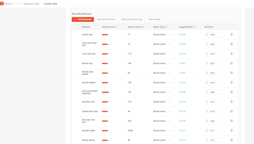
Selecting which keywords to bid for for keywords Ads in Shopee can be a hassle on Shopee platform. One of the main reason is that you cannot really sort or rank by the number of searches and/or bid price on Shopee platform. Having the option to export to excel/csv can really help on the analysis. And is really simple to do so with Python.

Navigate to the “Create (keyword) Ads”. Select Add Keywords and add as many related keywords as you like. Once completed, save the page as html file. Next we will use python pandas to parse the table tag in the html file and generate as pandas DataFrame.

## Sample Code
import pandas as pd

tgt = r'C:\yourfilelocation\shopee.html'

# list of table. 
# For this, table 0 is header col and table 1 is data
tb = pd.read_html(tgt) 

# Assign header from table 0 to table 1
tb[1].columns= tb[0].columns.tolist() 

# Drop empty columns
bid_table = tb[1].dropna(1,'all')     

# Can save to excel as well
bid_table.to_csv(r'c:\data\output.csv', index=False)

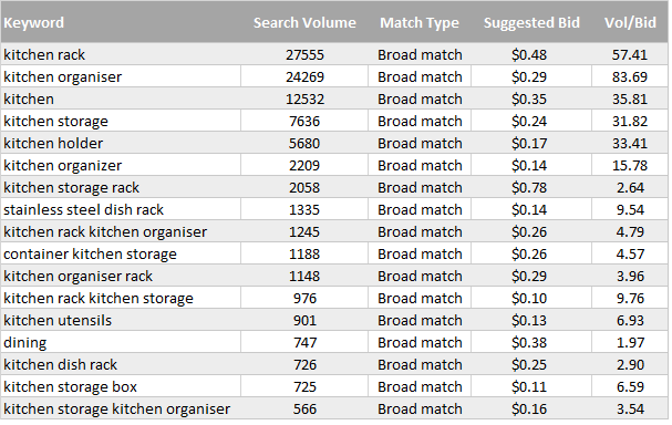
Sample of the output is shown above. I usually sort by search volume (highest). I also add in the Search Vol/Num Bids columns which give some indication of the search volume per 0.1cents of bids.

Selenium can be used to automated the saving of html file.

The “Quality Score” is not able to parse using the read_html method given it is a generated image file. However, for those who are really keen, the quality score is reflected in the image tag attribute [style=”width: x%]. Parsing this will give the the estimated quality score.

Simple way to export Shopee Ads keyword bids data to Excel using python pandas. https://simply-python.com/2021/04/19/export-shopeeads-keyword-bids/

Adding PostgreSQL to Django

Requirements

  1. VirtualEnv
  2. Django
  3. PostgreSQL

Add on to post from Painless PostgreSQL + Django

The recommendation is to follow the steps from the original well-written post and refers to the following to fill in some of the possible gaps .

  1. Activate a virtualenv
  2. Git clone the project (in the post) to local directory
  3. Run pip install -r requirements.txt
  4. Upgrade Django version (will encounter error if this step is not performed). pip install django==1.11.17.  This only applies if you following the post and cloning the project used in the post.
  5. Create new user in Postgres, create new database & grant assess (Step 1 & 2 of post)
  6. Update settings.py on the database portion.
  7. Create environment variables in the virtualenv.  See link for more information.
    1. Note: Secret Key needs to be included as one of the environment variable.
    2. Update the postactivate file of the virtualenv so the environment variables are present when virtualenv is activated.
    3. To get path of the virtualenv: echo $VIRTUAL_ENV

Create new user in Postgres

# Psql codes for Step 1 and 2 of original post.
# ensure Postgres server is running
psql
# create user with password
CREATE USER sample_user WITH PASSWORD 'sample_password';
# create database
CREATE DATABASE sample_database WITH OWNER sample_user;

Update database information in Setting.py

# Changes in the settings.py

DATABASES = {
    'default': {
        'ENGINE': 'django.db.backends.postgresql_psycopg2',
        'NAME': os.environ.get('DB_NAME', ''),
        'USER': os.environ.get('DB_USER', ''),
        'PASSWORD': os.environ.get('DB_PASS', ''),
        'HOST': 'localhost',
        'PORT': '5432',
    }
# SECURITY WARNING: keep the secret key used in production secret!
SECRET_KEY = os.environ.get('DJANGO_SECRET_KEY', '')

Update environment variables in VirtualEnv

# postactivate script in the project virtual env bin path.
# E.g. ~/.virtualenv/[projectname]/bin/postactivate

#!/bin/bash
# This hook is sourced after this virtualenv is activated.
export DB_NAME='sample_database'
export DB_USER='sample_user'
export DB_PASS='sample_password'
export DJANGO_SECRET_KEY='thisissecretkey'

Running migrations (Ensure PostgreSQL server is running)

python manage.py makemigrations
python manage.py migrate
python manage.py createsuperuser
python manage.py runserver

Additional notes:

  1. When running python manage.py runserver on local host and error occurs, check domain is included in the ALLOWED_HOSTS of setting.py. Alternatively, you can use below:
    • ALLOWED_HOSTS = [‘*’] # for local host only
  2. No database created when running psql command: CREATE DATABASE …, check if  semi-colon add to end of the statement. In the event, the ‘;’ is missing, type ‘;’ and try inputting the commands again. See link for more details.

Useful Seaborn plots for data exploration

Types of plots:

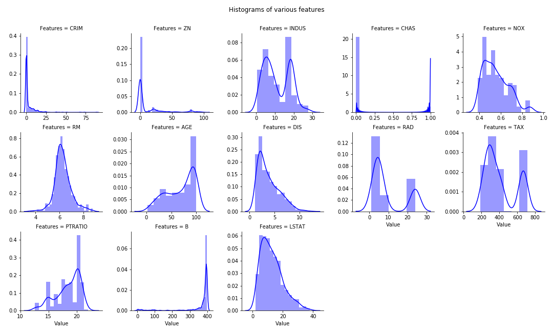
  1. Multiple features histogram in single chart
  2. Diagonal Correlation Matrix
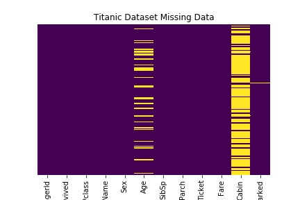
  3. Missing values Heat Map

Boston Housing prices dataset is used for 1, 2. Titanic Dataset for item 3.

Basic Python module import

import pandas as pd
import numpy as np
import seaborn as sns
import matplotlib.pyplot as plt
% matplotlib inline

from sklearn.datasets import load_boston
boston = load_boston()
X = boston.data
y = boston.target
df = pd.DataFrame(X, columns= boston.feature_names)

Multiple Histogram plots of numeric features

  • Stack the dataframe with all the features together. May consume significant memory if dataset have large number of features and observations.
  • If need to separate by group (hue in FacetGrid), can modify the numeric_features:
  • numeric_features= df.set_index(‘Group’).select_dtypes(exclude=[“object”,”bool”])
numeric_features= df.select_dtypes(exclude=["object","bool"])
numeric_features = numeric_features.stack().reset_index().rename(columns = {"level_1":"Features",0:"Value"})
g = sns.FacetGrid(data =numeric_features, col="Features",  col_wrap=5, sharex=False, sharey=False)
g = g.map(sns.distplot, "Value", color ='blue')
plt.subplots_adjust(top=0.9)
plt.suptitle("Histograms of various features")

multiplehist

Diagonal Heat Map of Correlation Matrix

Reference: seaborn.pydata.org. Utilize the Seaborn heat map with masking of the upper diagonal.

f, ax = plt.subplots(figsize=(12, 12))
corr = df.select_dtypes(exclude=["object","bool"]).corr()

# TO display diagonal matrix instead of full matrix.
mask = np.zeros_like(corr, dtype=np.bool)
mask[np.triu_indices_from(mask)] = True

# Generate a custom diverging colormap.
cmap = sns.diverging_palette(220, 10, as_cmap=True)

# Draw the heatmap with the mask and correct aspect ratio.
g = sns.heatmap(corr, mask=mask, cmap=cmap, vmax=1, center=0, annot=True, fmt='.2f',\
square=True, linewidths=.5, cbar_kws={"shrink": .5})

# plt.subplots_adjust(top=0.99)
plt.title("Diagonal Correlation HeatMap")

heatmap

Missing values Heat Map

Reference: Robin Kiplang’at github

dataset ='https://gist.githubusercontent.com/michhar/2dfd2de0d4f8727f873422c5d959fff5/raw/ff414a1bcfcba32481e4d4e8db578e55872a2ca1/titanic.csv'

titanic_df = pd.read_csv(dataset, sep='\t')
sns.heatmap(titanic_df.isnull(), yticklabels=False, cbar = False, cmap = 'viridis')

plt.title("Titanic Dataset Missing Data")

missingdata


Create own flash cards video using Python

Build your own study flash cards video (+ background music) using Python easily.

Required Modules

  1. moviepy
  2. ImageMagick — for creating text clip
  3. pandas — optional for managing CSV file

Basic steps

  1. Read in the text information. Pandas can be used to read in a .csv file for table manipulation.
  2. create a Textclip object for each text and append all Textclips together
  3. Add in an audio if desired.  Allow the audio to loop through duration of the clip
  4. Save the file as mp4.

Sample Python Project — Vocabulary flash cards

Below is a simple project to create a vocabulary list of common words use in GMAT etc. For each word and meaning pair, it will flash the word followed by its meaning . There is slight pause in the timing to allow some time for the user to recall on the meaning for the particular words

Sample table for wordlist.csv (which essentially is a table of words and their respective meanings) * random sample (subset) obtained from web

Screen Shot 2019-07-23 at 11.32.42 PM


def create_txtclip(tgt_txt, duration = 2, fontsize = 18):
    try:
        txt_clip = TextClip(tgt_txt, fontsize = fontsize, color = 'black',bg_color='white', size=(426,240)).set_duration(duration)
        clip_list.append(txt_clip)
    except UnicodeEncodeError:
        txt_clip = TextClip("Issue with text", fontsize = fontsize, color = 'white').set_duration(2)
        clip_list.append(txt_clip)

from moviepy.editor import *

df = pd.read_csv("wordlist.csv")
for word, meaning in zip(df.iloc[:,0], df.iloc[:,1]):
    create_txtclip(word,1, 70)
    create_txtclip(meaning,3)

final_clip = concatenate(clip_list, method = "compose")

# optional music background with loop
music = AudioFileClip("your_audiofile.mp3")
audio = afx.audio_loop( music, duration=final_clip.duration)

final_clip = final_clip.set_audio(audio)

final_clip.write_videofile("flash_cards.mp4", fps = 24, codec = 'mpeg4')<span id="mce_SELREST_start" style="overflow:hidden;line-height:0;"></span>

In some cases, the audio for the flash cards does not work when play with Quicktime, will work on VLC

Sample video (converted to gif)

ezgif.com-video-to-gif

PDF manipulation with Python

This post covers basic PDF manipulation for daily tasks using simple Python modules.

  1. Merging mulitple PDF
  2. Extract text from PDF
  3. Extract image from PDF

Merging PDF

from PyPDF2 import PdfFileMerger
pdfs = ['a.pdf', b.pdf]
merger = PdfFileMerger()

for pdf in pdfs:
    merger.append(pdf)

merger.write("output.pdf")

Extract text from PDF

import pdftotext

# Load your PDF
with open("Target.pdf", "rb") as f:
    pdf = pdftotext.PDF(f)

# Save all text to a txt file.
with open('output.txt', 'w') as f:
    f.write("\n\n".join(pdf))

More information from “Convert PDF pages to text with python

Extract Image (JPEG) from PDF


import os
import tempfile
from pdf2image import convert_from_path

filename = 'target.pdf'

with tempfile.TemporaryDirectory() as path:
     images_from_path = convert_from_path(filename, output_folder=path, last_page=1, first_page =0)

base_filename  =  os.path.splitext(os.path.basename(filename))[0] + '.jpg'      

save_dir = 'your_saved_dir'

for page in images_from_path:
    page.save(os.path.join(save_dir, base_filename), 'JPEG')

More information from “Convert PDF pages to JPEG with python

Google Colab import data, Specs, link Gsheets & link with Kaggle

Importing data to colab

  1. Direct import
    • from google.colab import files
      uploaded = files.upload()
    • import io
      df = pd.read_csv(io.BytesIO(uploaded[‘target.csv’]))
  2. Setup to use file from google drives
    • from google.colab import drive
      drive.mount(‘/content/drive’)
    • View list of files:
    • !ls “/content/drive/My Drive”
    • Note: In the notebook, click on the charcoal > on the top left of the notebook and click on Files, select the file and right click to “copy path”. Note the path must begin with “/content/xxx”

Hardware Spec for Colab

See link.

Linking with Google Sheets (reference from source)

# Step 1
!pip install --upgrade --quiet gspread

# Step 2
from google.colab import auth
auth.authenticate_user()

import gspread
from oauth2client.client import GoogleCredentials
gc = gspread.authorize(GoogleCredentials.get_application_default())

# Step 3
sh = gc.create('My spreadsheet')

worksheet = gc.open('My spreadsheet').sheet1

cell_list = worksheet.range('A1:C2')

import random
for cell in cell_list:
  cell.value = random.randint(1, 10)

worksheet.update_cells(cell_list)

Note: The google sheets is at the starting page of google Drive. Still figuring out the way to specify target directory.

Linking with Kaggle (eg. direct download and import Kaggle dataset)

  1. Retrieve API token from Kaggle (Kaggle–> accounts –> under AP,  hit “Create New API Token.”
  2. Save the token.json in Google Drive
  3. Run the following on colab to link with Kaggle
!pip install kaggle
!mkdir .kaggle
from googleapiclient.discovery import build
import io, os
from googleapiclient.http import MediaIoBaseDownload
from google.colab import auth

auth.authenticate_user()

drive_service = build('drive', 'v3')
results = drive_service.files().list(
        q="name = 'kaggle.json'", fields="files(id)").execute()
kaggle_api_key = results.get('files', [])

filename = "/content/.kaggle/kaggle.json"
os.makedirs(os.path.dirname(filename), exist_ok=True)

request = drive_service.files().get_media(fileId=kaggle_api_key[0]['id'])
fh = io.FileIO(filename, 'wb')
downloader = MediaIoBaseDownload(fh, request)
done = False
while done is False:
    status, done = downloader.next_chunk()
    print("Download %d%%." % int(status.progress() * 100))
os.chmod(filename, 600)

source: https://colab.research.google.com/drive/1JG6d49pAWpn4kF92c0Ko16gQV6hptAro#scrollTo=CSKDTkuLuTY3

!cp /content/.kaggle/kaggle.json ~/.kaggle/kaggle.json
!kaggle config set -n path -v{/content}

Testing

!kaggle datasets list

Downloading particular data set from Kaggle

  1. Under particular Kaggle competition, look under Data and get the API commands
  2. Eg. Some competition data set from Kaggle
  3. Commands copied from API: kaggle competitions download -c ndsc-advanced
  4. Modify the Command and run in Colab:
    • !kaggle competitions download -c ndsc-advanced -p /content
  5. Unzip the files:
    • !unzip \*.zip
  6. Open file with pandas:
    • import pandas as pd
      d = pd.read_csv(‘beauty_data_info_val_competition.csv’)

References:

  1. Setting Up Kaggle in Google Colab

Running R on Jupyter Notebook with R Kernel (No Anaconda)

A simple guide to install R Kernel on Jupyter Notebook (Windows).  Do not need Anaconda.

  1. Objectives:
      1. Install R Kernel on Jupyter Notebook (Windows)
  2. Required Tools:
      1. R for windows— R for windows
      2. JupyterNotebook — Jupyter Notebook
  3. Steps:
      1. Install R. Use the R terminal (do not use R studio) to install R packages:
        • install.packages(c(‘repr’, ‘IRdisplay’, ‘evaluate’, ‘crayon’, ‘pbdZMQ’, ‘devtools’, ‘uuid’, ‘digest’))
        • install.packages(‘IRkernel’)
      2. Make Kernel available to Jupyter
        • IRkernel::installspec()
        • OR IRkernel::installspec(user = FALSE) #install system-wide
      3. Open a notebook and open new R script.

Further notes 

  • After getting Additional R library might be hard to install inside the Notebook. For workaround, install desired library in R terminal then open the Notebook.
  • If need to use R.exe on windows command terminal, ensure R.exe is on path. [likely location: C:\R\R-2.15.1\bin]
  • ggplot tutorial

References:

Predict Product Attributes from Product Listings Part 2 – Pipelines & GridSearch

Further improvement on the Product Attributes Text Classifier

This is part 2 of the extracting attributes from product title with the following improvements or add on.

  1. Creating a more generic text cleaning function.
  2. Adding GridSearch for hyper parameters tuning.

Text Cleaning Function

I created a more generic text cleaning function that can accommodate various text data sets. This can use as a base function for text related problem set. The function, if enabled all options, will be able to perform the following:

  1. Converting all text to lowercase.
  2. Stripping html tags especially if data is scrapped from web.
  3. Replacing accented characters with closest English alphabets/characters.
  4. Removing special characters which includes punctuation. Digits may or may not be excluded depending on context. (Digits are not removed for this data set)
  5. Removing stop-words (simple vs detailed. If detailed, will tokenize words before removal else will use simple word replacement.
  6. Removing extra white spaces and newlines.
  7. Normalize text. This either refer to stemming or lemmatizing.

In this example, we only turn on:

  1. converting text to lowercase
  2. remove special characters (need to keep digits) and white spaces,
  3. do a simple stop words removal.

As mentioned in previous post, it is likely a seller would not include much stop words and will try to keep the title as concise as possible given the limited characters and also to make the title more relevant to search engine. As the text length is not too long, will skip normalizing text to save time.

# Text pre-processing modules
from bs4 import BeautifulSoup
import unidecode
import spacy, en_core_web_sm
nlp = spacy.load('en_core_web_sm', disable=['parser', 'ner'])
from nltk.corpus import stopwords
from nltk.tokenize import word_tokenize
from nltk.stem import PorterStemmer
STOPWORDS = set(stopwords.words('english')) 

# Compile regular expression
SPEC_CHARS_REPLACE_BY_SPACE = re.compile('[/(){}\[\]\|@,;]')
SPEC_CHARS = re.compile(r'[^a-zA-z0-9\s]')
SPEC_CHARS_INCLUDE_DIGITS = re.compile(r'[^a-zA-z\s]')
EXTRA_NEWLINES = re.compile(r'[\r|\n|\r\n]+')

## Functions for text preprocessing, cleaning

def strip_htmltags(text):
    soup = BeautifulSoup(text,"lxml")
    return soup.get_text()

def replace_accented_chars(text):
    return unidecode.unidecode(text)

def stem_text(text):
    ps = PorterStemmer()
    modified_txt = ' '.join([ps.stem(word) for word in text.split()])
    return modified_txt    

def lemmatize(text):
    modified_text = nlp(text)
    return ' '.join([word.lemma_ if word.lemma_ != '-PRON-' else word.text for word in modified_text])

def normalize(text, method='stem'):
    """ Text normalization to generate the root form of the inflected words.
        This is done by either "stem" or "lemmatize" the text as defined by the 'method' arguments.
        Note that using "lemmatize" will take much longer to run compared to "stem".
    """
    if method == 'stem':
        return stem_text(text)
    if method == 'lemmatize':
        return lemmatize(text)
    print('Please choose either "stem" or "lemmatize" method to normalize.')
    return text

def rm_special_chars(text, rm_digits=False):
    # remove & replace below special chars with space
    modified_txt = SPEC_CHARS_REPLACE_BY_SPACE.sub(' ', text)

    # remove rest of special chars, no replacing with space
    if rm_digits:
        return SPEC_CHARS_INCLUDE_DIGITS.sub('', modified_txt)
    else:
        return SPEC_CHARS.sub('', modified_txt)

def rm_extra_newlines_and_whitespace(text):
    # rm extra newlines
    modified_txt =  EXTRA_NEWLINES.sub(' ', text)

    # rm extra whitespaces
    return re.sub(r'\s+', ' ', modified_txt)

def rm_stopwords(text, simple=True):
    """ Remove stopwords using either the simple model with replacement.
        or using nltk.tokenize to split the words and replace each words. This will incur speed penalty.
    """
    if simple:
        return ' '.join(word for word in text.split() if word not in STOPWORDS)
    else:
        tokens = word_tokenize(text)
        tokens = [token.strip() for token in tokens]
        return ' '.join(word for word in tokens if word not in STOPWORDS)

def clean_text(raw_text, strip_html = True, replace_accented = True,
                normalize_text = True, normalize_methd = 'stem',
                remove_special_chars = True, remove_digits = True,
                remove_stopwords = True, rm_stopwords_simple_mode = True):

    """ The combined function for all the various preprocessing method.
        Keyword args:
            strip_html               : Remove html tags.
            replace_accented         : Convert accented characters to closest English characters.
            normalize_text           : Normalize text based on normalize_methd.
            normalize_methd          : "stem" or "lemmatize". Default "stem".
            remove_special_chars     : Remove special chars.
            remove_digits            : Remove digits/numeric as special characters.
            remove_stopwords         : Stopwords removal basedon NLTK corpus.
            rm_stopwords_simple_mode : skip tokenize before stopword removal. Speed up time.
    """

    text = raw_text.lower()

    if strip_html:
        text = strip_htmltags(text)
    if replace_accented:
        text = replace_accented_chars(text)
    if remove_special_chars:
        text = rm_special_chars(text, remove_digits)
    if normalize_text:
        text = normalize(text, normalize_methd)
    if remove_stopwords:
        text = rm_stopwords(text, rm_stopwords_simple_mode)

    text = rm_extra_newlines_and_whitespace(text)  

    return text

Grid Search for Hyper Parameters Tuning

Using pipelines, it is easy to incorporate the sklearn grid search to sweep through the various the hyper parameters and select the best value. Two main parameters tuning are:

  1. ngram range in CountVectorizer:
    • In the first part, we only looking a unigram or single word but there are some attributes that are identified by more than one word alone (eg 4G network, 32GB Memory etc) therefore we will sweep the ngram range to find the optimal range.
    • The larger the ngram range the more feature columns will be generated so it will be more memory consuming.
  2. alpha in SGDClassifier
    • This will affect the regularization term and the learning rate of the training model.

With the ngram range and alpha parameters sweep and the best value selected, we can see quite a significant improvement to the accuracy to all the attribute prediction compared to the first version. Most of the improvement comes from the ngram adjusted to (1,3), meaning account for trigram. This is within expectation as more attributes are described by more than one word.

# Prepare model -- Drop na and keep those with values
def get_X_Y_data(x_col, y_col):
    sub_df =  df[[x_col, y_col]]
    sub_df.head()
    sub_df = sub_df.dropna()
    return sub_df[x_col], sub_df[y_col]

# Model training & GridSearch
def generate_model(X, y, verbose = 1):

    text_vect_pipe = Pipeline([
                            ('vect', CountVectorizer()),
                            ('tfidf', TfidfTransformer())
                            ])

    pred_model = Pipeline([
                ('process', text_vect_pipe),
                ('clf', SGDClassifier(loss='hinge', penalty='l2',alpha=1e-3, random_state=42, max_iter=5, tol=None))
               ])

    parameters = {}
    parameters['process__vect__ngram_range'] = [(0,1),(1,2),(1,3)]
    parameters['clf__loss'] = ["hinge"]
    parameters['clf__alpha'] = [5e-6,1e-5]

    X_train, X_test, y_train, y_test = train_test_split(X, y, test_size=0.3, random_state = 42)

    CV = GridSearchCV(pred_model, parameters)
    CV.fit(X_train, y_train)
    y_pred = CV.predict(X_test)

    print('accuracy %s' % accuracy_score(y_pred, y_test))
    print("=="*18)
    print()
    print("Details of GridSearch")

    if verbose:
        print('Best score and parameter combination = ')
        print(CV.best_score_)
        print(CV.best_params_)
        print()
        print("Grid scores on development set:")
        means = CV.cv_results_['mean_test_score']
        stds = CV.cv_results_['std_test_score']
        for mean, std, params in zip(means, stds, CV.cv_results_['params']):
            print("%0.3f (+/-%0.03f) for %r"
                  % (mean, std * 2, params))
        print("=="*18)
        print()

    return CV

X, y = get_X_Y_data('title1', 'Brand')
brand_model = generate_model(X, y)
print('='*29)

The full script is as below. The text cleaning function takes a large part of the code. Excluding the function, the additional of few lines of code for the grid search and pipeline can can bring a relatively significant accuracy improvement.

Next Actions

So far only text features are considered, the next part we will try adding numeric features to see if further improvement can be made.

See Also

  1. Predict Product Attributes from Product Listing Title — Text Feature Extraction and Classification

Sorry, something went wrong. Reload?
Sorry, we cannot display this file.
Sorry, this file is invalid so it cannot be displayed.


Easy Create Mosaic Plot using Stacked Bar Chart

Creating Mosaic Plot

In one of my work project, I need to use mosaic plot to visualize the proportion of different variables/elements exists in each group.  It is hard to find a readily available mosaic plot function (from Seaborn etc) which can be easily customized. By reading some of the blogs, mosaic plot can be created using stacked bar chart concept by performing some transformation on the raw data and overlaying individual bar charts. With this knowledge and using python Pandas and Matplotlib, I am able to create a mosaic plot that is good enough for my need.

Sample Data Sets

A sample data set is as shown below. We need to plot the proportion of b, g, r (all the columns) for each index (0 to 4). Based on the format of the data set, we make a transformation of the columns to be able to have Mosaic Plot.

Sorry, something went wrong. Reload?
Sorry, we cannot display this file.
Sorry, this file is invalid so it cannot be displayed.

Breaking down the data transformation for stacked bar chart plotting

We perform two transformations as followed. Mosaic plot requires the sum of  proportion of categories for each group to be 1.0 or 100%. Stacked bar chart can achieve this by summing or stacking values for each element in the group but we would need to ensure the values are normalized and the sum of all elements in a group equal to 1 (i.e r+ g+b =1 for each index).

To simulate the effect of stacked bar chart , the trick is to use multiple bar charts to overlay on top of each other to simulate the effect of stacked bar chart. To be able to create the stacked effect, the ratio/proportion of the stacked element need to be the sum of proportion value of “bottom” elements + the proportion value of the element itself. This can be easily achieved by doing a cumulative sum along the row axis.

As example below, r will be used as a base (since values are based on b + g + r). g will overlay on top of r since it is summation of b + g. b will be final layer overlay on g and r.

Sorry, something went wrong. Reload?
Sorry, we cannot display this file.
Sorry, this file is invalid so it cannot be displayed.

Mosaic plot function

Once the transformations are done, it is easy to plot the mosaic plot by plotting the different bar charts and overlaying on top of each other. Additional module adjustText can be used to prevent overlapping of the text labels in the plot. Based on the above, we can create a general mosaic function as below.

Sorry, something went wrong. Reload?
Sorry, we cannot display this file.
Sorry, this file is invalid so it cannot be displayed.